Multiple shooting

This page provides an overview of multiple shooting in diff-soup. The recipe, data, and inference problem are those of fitting parameters.

An overview of multiple shooting

Suppose we have observations \(u_0, u_1, \dots, u_N\) of the state at the times \(t_0 < t_1 < \dots < t_N\) and a model with parameters \(\theta\). A single-shooting fit integrates the model from \(u_0\) over the whole horizon \([t_0, t_N]\) and minimizes the misfit \(\sum_n \|\hat u(t_n;\theta) - u_n\|^2\) over \(\theta\). Every observation is then predicted through one long solve, so a poor starting guess drifts away from the data along the horizon, as in the left panel below.

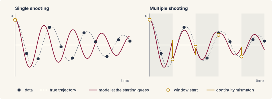
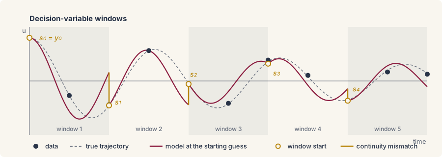
Multiple shooting partitions the horizon into windows \([\tau_{w-1}, \tau_w]\), \(w = 1, \dots, W\), and integrates each window from its own start state \(s_{w-1}\), with \(s_0 = u_0\). The window starts join \(\theta\) as decision variables, and the loss adds a continuity term that pulls the end of each window to the start of the next. Writing \(\Phi(s;\theta)\) for the state a window reaches when it starts from \(s\),

\[ \min_{\theta,\, s_1, \dots, s_{W-1}}\; \sum_n \|\hat u_w(t_n;\theta, s_{w-1}) - u_n\|^2 \;+\; \sum_{w=1}^{W-1} \big\|s_w - \Phi(s_{w-1};\theta)\big\|^2_{W_c}, \]

where each observation is predicted on the window \(w\) that contains \(t_n\) and \(W_c\) weights the continuity term. At the solution the mismatches vanish and the windows join into one trajectory.

Two window modes

ds.inference.Multishoot(windows, continuity=None, states=None) is passed as ds.inference.Experiment(trajectory=), or as ds.inference.InferenceProblem(trajectory=) to apply it to every experiment, and the windows constructor selects the mode.

• ds.inference.Windows.from_data(source=None) starts every window from a measured state, one window per consecutive pair of frames. Only the parameters are fitted, and there is no continuity term. This needs a data stream that observes the full state, named by source= when there are several.

experiment = ds.inference.Experiment(problem, solver, (0.0, 0.1), y0, (measurement,),
                                     trajectory=ds.inference.Multishoot(ds.inference.Windows.from_data(source="u")))
infproblem = ds.inference.InferenceProblem(experiment, parameters=D)
infproblem.n_segments      # 4, one window per consecutive pair of frames
result = ds.inference.optsolve(infproblem)
result[D]            # 0.298
result.diagnostics.per_series_cost   # one cost per window

infproblem.n_segments is the window count, and result.diagnostics.per_series_cost holds one cost per window. A measurement with the default readout (no observe=) seeds the windows, and a partial readout is refused.

• ds.inference.Windows.at(ts) places window boundaries at the times ts, from the initial time to the last frame, and fits the window starts beside the parameters. ds.inference.Windows.uniform(n) places n equal windows over the same horizon.

windows = ds.inference.Windows.at(jnp.concatenate([jnp.array([0.0]), ts]))
experiment = ds.inference.Experiment(problem, solver, (0.0, 0.1), y0, (measurement,),
                                     trajectory=ds.inference.Multishoot(windows, ds.inference.Continuity(weight="auto")))
infproblem = ds.inference.InferenceProblem(experiment, parameters=D)
infproblem.n_params        # 121, one diffusivity and four window starts of 30 differential values
result = ds.inference.optsolve(infproblem)
result[D]            # 0.2993
result.window_states.shape               # (4, 30)
result.diagnostics.window_obs_rank       # (30, 30, 30, 30)
result.diagnostics.continuity_defect_wrms   # one defect per window, in state units

The window starts are initialized from one solve at the starting parameters. With few probes of a large state, the data inside a window determine only some of its start values; the rest are held by the continuity rows and stay near that first solve, so multiple shooting does not by itself rescue a start the single shot cannot. result.window_states holds their fitted values, and result.params leads with the parameters. For a DAE, only the differential part of the state is fitted per window and the algebraic part is recovered from it (consistent initialization).

ds.inference.NewtonTrustRegion steps on the Gauss-Newton matrix here, as it does for every fit with residual rows (solvers). The memory of the exact Hessian grows with the square of the decision vector, and a few hundred entries can already exceed the device.

Options

The options, with their defaults:

• continuity=ds.inference.Continuity(weight="auto") weights the continuity term at the scale of the data misfit, from the solver's tolerances and the observation weights. A positive float weight=W weights every continuity row by \(\sqrt{W}\) instead.
• states=ds.inference.StateBasis.full() fits every differential entry of a window start. ds.inference.StateBasis.from_modes(B) fits only a coefficient vector in the column-orthonormal basis B, which shrinks the decision vector when the state is large.

Batching and derivatives

• Each window is solved once per evaluation, saving its frames on the way, so a fit integrates the horizon once however many frames a window holds.
• A window's solve reads only the parameters and its own start. Its Jacobian therefore pushes one tangent per parameter and one per entry of a window start through all the windows at once, not one per decision variable.
• The windows solve as one batch. A jax.vmap over parameter values of the likelihood joins that batch, and so do the chains of ds.inference.sample.
• jax.grad of the likelihood runs with the solver's reverse adjoint, ds.CheckpointAdjoint() by default. Take the gradient of a function that calls the likelihood, not of a jax.jit around it.

Reading the result

• result.diagnostics.continuity_defect_wrms gives, per window, the root mean square of the continuity mismatch in state units. At a good solution every entry is small.
• result.diagnostics.window_obs_rank gives, per window, how many directions of the window start the data inside that window determine, and an under-determined window is noted in warnings.
• result.diagnostics.continuity_unrepresented gives, per window, the mismatch a reduced StateBasis cannot represent, and the diagnostics carry a note to widen the basis when it is large.
• A decision vector beyond 2000 entries warns that the dense Gauss-Newton solve is the cost wall. The exact Hessian reaches its wall far earlier, and a fit that would exceed the device memory stops before it starts with an error naming hessian_tile=.
• Windows with fitted starts take exactly one measurement. A second measurement is refused.
• ds.inference.Experiment(..., initial_state=ds.inference.LearnedInitialState(guess)) adds the start of the first window to the decision vector (data assimilation).