Hierarchical fits¶

This page provides an overview of fitting several experiments together, with parameters shared across all of them, tied within clusters of experiments, or local to each experiment. Throughout, we fit synthetic data from three electrode particles, each run under a potentiostatic and a galvanostatic protocol. We recover a shared diffusivity and a per-particle rate constant.

The particle model¶

Each particle is a sphere of radius \(R\) in which the lithium filling fraction \(c \in (0, 1)\) diffuses,

\[ \frac{\partial c}{\partial t} = D\,\nabla^2 c, \qquad r \in (0, R), \]

with the intercalation flux into the particle at the surface given by Butler-Volmer kinetics against the ideal-solution open-circuit potential, in units of the thermal voltage,

\[ j(c_s, V) = k\,\sqrt{c_s (1 - c_s)}\,\big(e^{-\eta/2} - e^{\eta/2}\big), \qquad \eta = V - \ln\frac{1 - c_s}{c_s}, \]

where \(c_s\) is the surface fraction, \(V\) the applied potential, and \(k\) the rate constant. Under the potentiostatic protocol \(V\) is held at a fixed value. Under the galvanostatic protocol the total current \(4 \pi R^2 j\) is held at a fixed value and \(V\) is the algebraic unknown that closes it (constraints). Simplifying the expression, the flux is \(j = k\,[(1 - c_s)\,e^{-V/2} - c_s\,e^{V/2}]\), the form the recipe evaluates. The recipe works in nanometers and seconds, and is a template (recipe templates) whose arguments are the radius and the protocol, so that one declaration serves every particle:

n = 24


def intercalation_flux(c_s, V, k):
    return k * ((1.0 - c_s) * jnp.exp(-V / 2) - c_s * jnp.exp(V / 2))   # Butler-Volmer against the ideal OCV


@ds.recipe
def particle(R=100.0, protocol="potentiostatic"):
    spec = ds.problem(f"particle_{protocol}")
    spec.domain("particle", spherical_grid_1d(n, R, method="fvm"))
    spec.field("c", mass="differential", scale=1.0)
    spec.param("D", value=3e3, learnable=True, bounds=(1e2, 1e6))   # nm^2 / s, shared by every particle
    spec.param("k", value=10.0, learnable=True, bounds=(0.1, 1e3))  # nm / s, one value per particle

    @spec.equation(writes="c", reads=("c",))
    def diffusion(q):
        return q.p.D * q.ops.laplacian(q.c)

    if protocol == "potentiostatic":
        spec.control.potentiostatic(name="V", fn=lambda t: -2.0)
        spec.bc.flux("c", node_indices=np.array([n - 1]), fn=lambda q, t: intercalation_flux(q.c, q.control.V, q.p.k))
    else:
        spec.global_var("V", initial=-1.0)
        spec.bc.flux("c", node_indices=np.array([n - 1]), fn=lambda q, t: intercalation_flux(q.c, q.V, q.p.k))
        spec.constraint.galvanostatic(
            name="current", closes="V",
            current_fn=lambda q: 4 * jnp.pi * R**2 * intercalation_flux(q.c[n - 1], q.V, q.p.k),
            target_fn=lambda t: 4 * jnp.pi * R**2 * R / 12.0)
    return spec


D = particle.handle("D")
k = particle.handle("k")

Particle A has \(R = 100\) nm and \(k = 30\) nm/s, particle B has \(R = 200\) nm and \(k = 15\) nm/s, particle C has \(R = 150\) nm and \(k = 20\) nm/s, and all three share \(D = 10^4\) nm\(^2\)/s. The six experiments are solved at those values and sampled at ten times with noise of scale \(10^{-3}\). Every particle starts at \(c = 0.2\):

solver = ds.JIDA()
ts = jnp.linspace(0.2, 2.0, 10)
particles = {"A": 100.0, "B": 200.0, "C": 150.0}
k_true = {"A": 30.0, "B": 15.0, "C": 20.0}
experiments = []
for label, R in particles.items():
    for protocol in ("potentiostatic", "galvanostatic"):
        problem = particle.build(R=R, protocol=protocol)
        y0 = problem.assemble_state({"c": 0.2})
        theta_true = ds.default_theta(problem, {D: 1e4, k: k_true[label]})
        sol = ds.pdesolve(problem, solver, (0.0, 2.0), y0, theta=theta_true, saveat=ds.SaveAt(ts=ts))
        data = sol.ys + 1e-3 * np.random.default_rng(len(experiments)).standard_normal(sol.ys.shape)
        experiments.append(ds.inference.Experiment(
            particle, inputs={"R": R, "protocol": protocol}, id=f"{label}-{protocol}",
            solver=solver, t_span=(0.0, 2.0), initial_state=y0, parameters={"particle": label},
            measurements=(ds.inference.Measurement("c", ts, data, likelihood=ds.inference.Gaussian(sigma=1e-3)),)))

The hierarchical least-squares problem¶

Here we parameterize the solution of experiment \(i\), \(\hat u_i(\theta_s, \theta_{k(i)}, \theta_i)\), with three tiers of learnable parameters: \(\theta_s\) shared across every experiment, \(\theta_k\) tied within the cluster \(k(i)\) that experiment \(i\) belongs to, and \(\theta_i\) local to experiment \(i\). The shared tier holds the physics common to every experiment, such as a material's diffusivity. A cluster holds what a group of experiments has in common, such as the geometry of one particle run under several protocols. The local tier holds what belongs to one experiment alone, such as a quantity specific to its protocol. Given the observed data \(u_{\text{data}, i}\) of each experiment, we fit every tier at once by minimizing the joint least-squares loss

\[ \mathcal{L} = \tfrac{1}{2} \sum_{i=1}^{N} \big\| \hat u_i(\theta_s, \theta_{k(i)}, \theta_i) - u_{\text{data}, i} \big\|_2^2 . \]

In our example \(\theta_s = D\), the clusters are the three particles with \(\theta_A = k_A\), \(\theta_B = k_B\), and \(\theta_C = k_C\), each cluster holding one potentiostatic and one galvanostatic experiment, and the local tier is empty. The joint decision vector is ordered \([\theta_s \mid \theta_A\, \theta_B \cdots \mid \theta_1 \cdots \theta_N]\).

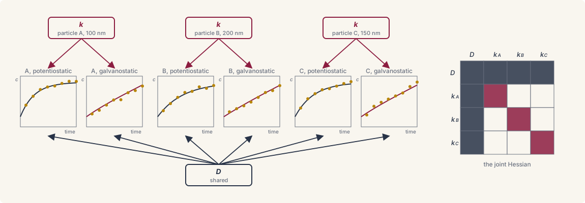
The parameter tiers, the experiments each parameter enters, and the arrowhead pattern of the joint Hessian

Each experiment couples only to the shared block and to its own cluster, so the Jacobian and the Hessian of the loss have an arrowhead structure, one block per cluster bordered by the shared block. ds.inference.TrustRegion factors that structure cluster by cluster and solves the shared block last, so the joint Hessian is never assembled.

The full fit:

hierarchy = ds.inference.Hierarchy(levels=("particle",), shared=(D,), per={"particle": (k,)})
study = ds.inference.Study(experiments, parameters=hierarchy)
lowered = ds.lower(study)
result = ds.inference.optsolve(lowered, ds.inference.TrustRegion())
result[D]            # the shared diffusivity
result[k]["A"]       # the rate constant of particle A
result[k]["B"]       # the rate constant of particle B
result[k]["C"]       # the rate constant of particle C

Solving the hierarchical least-squares problem¶

To solve this problem, we declare one ds.inference.Experiment per experiment, tie their parameters together in a ds.inference.Study through a ds.inference.Hierarchy, lower the study with ds.lower, and solve it using ds.inference.optsolve with ds.inference.TrustRegion().

Declare the experiments¶

Each experiment is declared as on fitting parameters, with the template in place of a built problem and its arguments under inputs=.

experiments.append(ds.inference.Experiment(
    particle, inputs={"R": R, "protocol": protocol}, id=f"{label}-{protocol}",
    solver=solver, t_span=(0.0, 2.0), initial_state=y0, parameters={"particle": label},
    measurements=(ds.inference.Measurement("c", ts, data, likelihood=ds.inference.Gaussian(sigma=1e-3)),)))

model is the template. inputs= gives the arguments of this experiment's build, and the experiment builds the recipe for them.
inputs= may also name a declared parameter, fixing its value for this experiment alone. A parameter that is fixed here and fitted through parameters= is refused.
id= names the experiment in the result and in the reports. The default is built from inputs=.
parameters= names the experiment's member of each level of the hierarchy, here the particle it belongs to.
A built problem is accepted in place of the template, with the handles of any one build. A handle is matched to each experiment's declaration by name, and a declaration whose size or learnable= flag differs between experiments is refused.

Pose the joint inference problem¶

ds.inference.Hierarchy declares which parameters are shared and which take one value per member of a level, ds.inference.Study ties the experiments to it, and ds.lower prepares the study for fitting (pose the inference problem).

hierarchy = ds.inference.Hierarchy(levels=("particle",), shared=(D,), per={"particle": (k,)})
study = ds.inference.Study(experiments, parameters=hierarchy)
lowered = ds.lower(study)

levels= names the levels between the study and its experiments, outermost first. Here the one level is the particle.
shared= lists the handles with one value for the whole study.
per= maps a level name to the handles that take one value per member of that level. The key "experiment" places a handle with one value per experiment.
The experiments that name the same member share its value. The joint coordinates are named by member, k@A and k@B, in the reports.
Bounds are those declared on the handle in each experiment, and a tied handle declares the same bounds in every experiment (box bounds).
layout= on ds.lower places the experiments across several devices (multi-GPU parallelism).
lowered.n_params is the length of the joint decision vector.

Run the fit¶

ds.inference.TrustRegion() is the recommended optimizer for a hierarchical study. It is a trust-region Gauss-Newton method solved level by level. The curvature is assembled one cluster at a time from that cluster's experiments, and each step is solved from the clusters up to the shared parameters.

result = ds.inference.optsolve(lowered, ds.inference.TrustRegion())

The options, with their defaults:

hessian="gauss-newton" uses the Gauss-Newton curvature, and "true" the exact Hessian.
max_steps=30 bounds the number of steps. target_accepted_steps=None, when set, ends the run after that many accepted steps with the status ACCEPTED_STEPS.
nested_at=None names a level at which the fit splits into two loops. The levels above it take the outer step, and each member of that level then refits its own parameters.
radius_init=, radius_max=, eta=, grad_tol=, step_tol=, cost_tol=, and x_scale= are the trust-region options of ds.inference.NewtonTrustRegion (Newton trust region).
weights=None gives one nonnegative weight per cluster, multiplying that cluster's contribution to the loss.
constraints=() and gauges=() add linear equality constraints on the joint vector, LinearConstraint and Gauge from diff_soup.inference.statistics.parameters. A gauge pins a direction the data leave free, such as the mean of a spatial field.
fixed_indices=() freezes the joint coordinates at those indices.
callbacks=() attaches callbacks to the solver (run the fit).
ds.inference.optsolve(lowered, ..., checkpoint=directory) saves the fit after every attempt and, when the directory already holds one, resumes from the newest.

ds.inference.NewtonTrustRegion() and ds.inference.LevenbergMarquardt() also fit a lowered study, by dense steps over the whole joint vector. TrustRegion is the best choice when the joint vector is large, since its curvature stays cluster-local.

Analyze the result¶

The result object carries the fields of a single fit (analyze the result) with the joint structure on top.

result[D]                                     # the shared diffusivity
result[k]                                     # {"A": ..., "B": ..., "C": ...}, one value per cluster
result.experiments["A-potentiostatic"][k]     # the value that experiment used
result.experiments["A-potentiostatic"].opt_params

result[D] returns the fitted value of a shared handle, and result[k] a dictionary from cluster label to the fitted value of a varying handle.
result.experiments holds one entry per experiment by its id, with [handle] the value that experiment used, and opt_params the experiment's parameters in the form ds.pdesolve takes through theta=.
result.params is the joint decision vector, shared handles first.

Uncertainty across the population¶

The uncertainty methods of statistical estimation and identifiability take the joint problem and its fit, and index their results by handle and by cluster label. The population methods estimate the spread of a parameter across the clusters:

posterior = ds.inference.laplace(lowered, result)
posterior[D].sd                                      # the standard error of the shared diffusivity
posterior[k]["A"].sd                                 # the standard error of the rate constant of particle A
posterior.cov[D, k][None, "A"]                       # the covariance of D with k of particle A

robust = ds.inference.cluster_covariance(lowered, result, cluster="particle")
boot = ds.inference.bootstrap(lowered, result, replicates=100, key=jax.random.key(0))
boot.interval(D)                                     # the bootstrap interval of the shared diffusivity
prof = ds.inference.profile(lowered, result, k, owner="A", optimizer=ds.inference.TrustRegion(), max_steps=8)
prof.interval(0.95)                                  # the profile interval of the rate constant of particle A

ds.inference.laplace(problem, fit) is the Laplace approximation of the joint posterior. posterior[D] is the marginal of a shared handle, posterior[k]["A"] the marginal of a varying handle in one cluster, and posterior.cov[D, k] a dictionary of covariances keyed by the pair of cluster labels, None for a shared handle.
ds.inference.cluster_covariance(problem, fit, *, cluster) estimates the covariance of the fit from the spread of the residuals between the clusters of cluster, without trusting the declared noise scale.
ds.inference.bootstrap(problem, fit, *, replicates, key) refits the study replicates times with the clusters reweighted, and boot[handle] returns the fitted values across the replicates. It refuses fewer than three clusters, naming the count and the minimum. steps=3 is the number of accepted trust-region steps each replicate takes from the fit, and steps="refit" refits each replicate to convergence. checkpoint= saves the run to a directory, and a later call with the same arguments resumes from it.
ds.inference.profile(problem, fit, handle, *, owner=, optimizer=) walks one cluster's value of a varying handle, named by owner=, with every other parameter refitted by ds.inference.TrustRegion (the profile likelihood).