Identifiability

This page provides an overview of determining practical identifiability of fitted parameters given the dataset. Throughout, we fit synthetic data generated by solving the heat equation of statistical estimation with a source term,

\[ \frac{\partial u}{\partial t} = D\,\frac{\partial^2 u}{\partial x^2} + a, \qquad x \in (0, 1), \]

with \(u(0, t) = u_0 = 0\), \(u(1, t) = u_1 = 1\), \(u(x, 0) = x\), \(D = 0.3\), and \(a = 1\), observed at five times between \(t = 0.05\) and \(t = 1.5\) with noise of scale \(10^{-1}\). Over that window the solution approaches the steady state

\[ u = -\frac{a}{2D}\,x^2 + \Big(u_1 - u_0 + \frac{a}{2D}\Big)\,x + u_0, \]

which depends on the diffusivity and the source amplitude only through \(a / D\), so that the two can trade off against each other:

import jax

jax.config.update("jax_enable_x64", True)

import jax.numpy as jnp
import numpy as np

import diff_soup as ds
from diff_soup.domains import cartesian_grid_1d

n = 32
spec = ds.problem("heat_source")
spec.domain("rod", cartesian_grid_1d(n, 0.0, 1.0, method="fvm"))
spec.field("u", mass="differential", scale=1.0, init=lambda x: x)
spec.param("D", value=0.3)                                            # the generating diffusivity
spec.param("a", value=1.0)                                            # the generating source amplitude


@spec.equation(writes="u", reads=("u",))
def heat(q):
    return q.p.D * q.ops.laplacian(q.u) + q.p.a


spec.bc.dirichlet("u", node_indices=np.array([0]), value=0.0)
spec.bc.dirichlet("u", node_indices=np.array([n - 1]), value=1.0)
problem_true = spec.build()
y0 = spec.assemble_state({})
solver = ds.JIDA()

ts = jnp.array([0.05, 0.15, 0.3, 0.5, 1.5])
sol_true = ds.pdesolve(problem_true, solver, (0.0, 1.5), y0, saveat=ds.SaveAt(ts=ts))
data = sol_true.ys + 1e-1 * np.random.default_rng(0).standard_normal(sol_true.ys.shape)

The practical identifiability problem

A parameter is structurally identifiable when it can be uniquely determined from noiseless data. Structural identifiability is out of scope for diff-soup.

A parameter is practically identifiable when it can be determined up to a given precision from noisy data.

Here we fit the two parameters \(\theta = (D, a)\) through maximum likelihood estimation (statistical estimation). Physically, we observe the rod gradually heat to the quadratic profile, but the noisy data can be explained both through a reaction-dominated mechanism (left panel) and through a diffusion-dominated mechanism (middle panel).

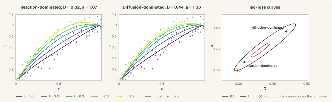
As shown in the iso-loss curves, the high noise level induces a degeneracy in the loss surface that shows up as an elongated diagonal stretch. This model problem demonstrates the practical identifiability problem, since many plausible parameter combinations explain the data.

To address this problem, we can analyze the Fisher information matrix

\[ \mathrm{FIM} = S^\top \Sigma^{-1} S , \]

where \(S\) is the sensitivity of the predicted data to the parameters and \(\Sigma\) the covariance of the measurement noise.

The eigendecomposition and null space provide valuable information about the inference problem. The eigenvalues describe the curvature of the iso-loss surface, and the condition number, the ratio of the largest to the smallest eigenvalue, gives a quantitative metric for how identifiable the parameters are. The eigenvectors describe the correlation structure of the parameters. The null space describes the exact degeneracy of parameters.

In diff-soup we calculate the Fisher information matrix and compute its condition number with ds.inference.identifiability, and we get a comprehensive diagnostic profile with ds.inference.profile, which fixes the \(j\)-th parameter at each value of a grid, refits the likelihood over the other parameters, and reads the confidence interval off the values where the profiled negative log likelihood stays within \(\tfrac{1}{2}\chi^2_{1,\alpha}\) of its minimum. The full analysis:

spec = ds.problem("heat_source")
spec.domain("rod", cartesian_grid_1d(n, 0.0, 1.0, method="fvm"))
spec.field("u", mass="differential", scale=1.0, init=lambda x: x)
D = spec.param("D", value=0.1, learnable=True, bounds=(0.01, 2.0))      # the learnable diffusivity
a = spec.param("a", value=0.5, learnable=True, bounds=(0.0, 5.0))       # the learnable source amplitude


@spec.equation(writes="u", reads=("u",))
def heat(q):
    return q.p.D * q.ops.laplacian(q.u) + q.p.a


spec.bc.dirichlet("u", node_indices=np.array([0]), value=0.0)
spec.bc.dirichlet("u", node_indices=np.array([n - 1]), value=1.0)
problem = spec.build()
y0 = spec.assemble_state({})

measurement = ds.inference.Measurement("u", times=ts, values=data,
                                       likelihood=ds.inference.Gaussian(sigma=1e-1))
experiment = ds.inference.Experiment(model=problem, solver=solver, t_span=(0.0, 1.5),
                                     initial_state=y0, measurements=(measurement,))
est = ds.inference.InferenceProblem(experiment, parameters=(D, a))
fit = ds.inference.optsolve(est, ds.inference.LevenbergMarquardt())                     # the maximum-likelihood fit

ident = ds.inference.identifiability(est, fit)                                          # the information spectrum at the fit
ident.raw.condition_number                                                              # the ratio of the largest to the smallest eigenvalue
prof = ds.inference.profile(est, fit, D, levels=(0.95,))                                # the profile likelihood of D
prof.interval(0.95)                                                                     # the 95% confidence interval of D

Analyzing identifiability

The fit is the maximum-likelihood fit of statistical estimation with two handles. The analysis then takes the inference problem and its fit.

The information spectrum

ds.inference.identifiability(problem, fit, *, parameter_scales=None, ridge=1e-10, null_tol=1e-10) computes the information matrix at the fit and reports its spectrum. For a MAP fit the prior is left out, so that a prior cannot hide a direction the data leaves open.

ident = ds.inference.identifiability(est, fit)
ident.names                              # ("D", "a")
ident.raw.condition_number               # the ratio of the largest to the smallest eigenvalue
ident.raw.sensitivity_rank               # the number of directions the data determine
ident.raw.null_directions                # the directions the data do not see, empty here
ident.scaled.eigenvalues                 # the spectrum after scaling each parameter

• fit is the fit result, or a mapping from handle to value, {D: 0.3, a: 1.0}, to analyze another point.
• parameter_scales= gives one scale per parameter, {D: 0.1, a: 1.0}, so that parameters of different units compare. The default scales every parameter by one. ident.raw is the spectrum in the parameters' own units, and ident.scaled the spectrum after the scaling.
• null_tol= is the fraction of the largest eigenvalue below which a direction counts as unseen and is listed in null_directions, each with its eigenvalue, its loadings on the parameters, and a description in words.
• ridge= regularizes the correlation matrix of the report only.
• Each of ident.raw and ident.scaled carries eigenvalues, loadings, correlation, condition_number, sensitivity_rank, null_directions, and notes.

The profile likelihood

ds.inference.profile(problem, fit, handle, *, owner=None, optimizer=None, levels=(0.95,), bounds=None, max_steps=24, multistart=0, multistart_scale=1.0) walks one parameter away from the fit in both directions, refitting every other parameter at each step, until the negative log likelihood has risen past the threshold of every level:

prof = ds.inference.profile(est, fit, D, levels=(0.95,), max_steps=24)
prof.interval(0.95)      # the lower and upper bounds of the 95% interval
prof.threshold(0.95)     # half the chi-squared quantile with one degree of freedom
prof.grid                # the values of D the walk visited
prof.delta_nll           # the rise of the negative log likelihood at each of them
prof.open_directions     # the sides that never reached the threshold, empty here

• handle is the parameter to profile, a scalar handle returned by spec.param. A parameter with one value per cluster takes owner= (hierarchical fits). A function handle is refused.
• levels= lists the confidence levels the walk covers, and prof.interval(level) returns the lower and upper bounds at one of them. An open side is reported as inf.
• max_steps= caps the number of steps per side.
• bounds=(lo, hi) narrows the range of the walk. The bounds declared on the handle apply as well, and a side the walk cannot cross within them is open.
• multistart= refits each step from that many perturbed starts, with multistart_scale= the size of the perturbation. The default refits from the previous step.
• optimizer= is the refitting algorithm. The default is ds.inference.LevenbergMarquardt(). A hierarchical study also accepts ds.inference.TrustRegion() (hierarchical fits). Any other algorithm is refused.
• A fit that did not converge is refused. A MAP fit profiles the posterior objective instead, and its intervals carry no coverage guarantee.
• A multiple-shooting fit that fits its window starts is refused. Refit with single shooting from its parameters and profile that fit.

Sensitivity runs

The information matrix is built from the sensitivity \(S\) of the solution to the parameters. ds.inference.sensitivity_solve(problem, t_span, y0, *, wrt, saveat, solver=None) computes it directly for a built problem, before any data exists, which is how an experiment is judged before it is run:

run = ds.inference.sensitivity_solve(problem, (0.0, 1.5), y0, wrt=(D, a),
                                     saveat=ds.SaveAt(ts=ts), solver=solver)
S = run.sensitivities()      # the sensitivity of every saved value to D and to a
run.x0                       # the parameter values the sensitivities are taken at

• wrt= is the tuple of handles the sensitivities are taken with respect to.
• saveat= gives the times the sensitivities are saved at, and solver= the time-stepping solver (ODE/DAE solvers).
• run.sensitivities(x=None) returns the sensitivities at the parameter values x, the declared values by default, and run(x) returns the saved solution values there. The run solves in the forward sensitivity mode of sensitivities and autodiff.

The practical identifiability report

ds.inference.practical_report(problem, fit, *, posterior=None, profiles=(), tolerances=None, report=None, experiment_id=None) collects the evidence of this page in one object. It carries the information spectrum at the fit, a summary of each supplied profile, the standard errors of a supplied Laplace approximation, and the residual report of goodness of fit. It states no overall verdict:

posterior = ds.inference.laplace(est, fit)
practical = ds.inference.practical_report(
    est, fit, posterior=posterior, profiles=(prof,), tolerances={"D": 0.01, "a": 0.1})
practical.local_sensitivity.raw.condition_number   # the spectrum at the fit
practical.likelihood_geometry                   # one summary per supplied profile
practical.status                                # one pass or fail per named tolerance
practical.provenance["missing_evidence"]        # the sections not supplied, none here

• posterior= is the Laplace approximation of standard errors and covariance.
• profiles= is a tuple of profile results.
• tolerances= maps a parameter name to the largest standard error it may have, and each status entry compares the standard error of the supplied posterior against that number. A tolerance without a posterior is refused.
• report= reuses an identifiability report already computed at this fit, and experiment_id= selects the experiment of the residual report when several are fitted together.

Function-valued parameters

A learnable function of function approximation is fitted through its coefficients, and its identifiability is a question about the function rather than about any one coefficient. ds.inference.function_report(information, block, *, gram=None) takes the coefficients of one function out of an information matrix, eliminates the other parameters, and reports the eigenvalues against the function's own norm. For the Legendre diffusivity of function approximation fitted as an inference problem est_f with the fit fit_f:

from diff_soup.inference.approx import Legendre

info_f = ds.inference.information(est_f, at=fit_f)
gram = Legendre(jnp.asarray(fit_f.params), interval=(0.0, 1.0)).gram()
report_f = ds.inference.function_report(info_f, "D_of_x", gram=gram)
report_f.eigenvalues      # the information per unit of the function's squared norm, one per mode
report_f.names

• block names the function handle.
• gram= is the Gram matrix of the function's basis, from the basis object's gram().