Posterior sampling

This page provides an overview of sampling the posterior of a statistical fit with ds.inference.sample. Throughout, we sample the posterior of an adsorption-diffusion model, a rod that loses solute to a saturating sink,

\[ \frac{\partial u}{\partial t} = D\,\frac{\partial^2 u}{\partial x^2} - a\,\frac{u}{1 + u}, \qquad x \in (0, 1), \]

with \(u(0, t) = 0\), \(u(1, t) = 1\), \(u(x, 0) = x\), \(D = 0.3\), and \(a = 1\), observed at five times between \(t = 0.05\) and \(t = 1.5\) with noise of scale \(10^{-1}\), and with a normal prior on each of the two parameters:

import jax

jax.config.update("jax_enable_x64", True)

import jax.numpy as jnp
import numpy as np

import diff_soup as ds
from diff_soup.domains import cartesian_grid_1d

n = 32
spec = ds.problem("adsorption")
spec.domain("rod", cartesian_grid_1d(n, 0.0, 1.0, method="fvm"))
spec.field("u", mass="differential", scale=1.0, init=lambda x: x)
spec.param("D", value=0.3)                                            # the generating diffusivity
spec.param("a", value=1.0)                                            # the generating adsorption rate


@spec.equation(writes="u", reads=("u",))
def adsorption(q):
    return q.p.D * q.ops.laplacian(q.u) - q.p.a * q.u / (1.0 + q.u)


spec.bc.dirichlet("u", node_indices=np.array([0]), value=0.0)
spec.bc.dirichlet("u", node_indices=np.array([n - 1]), value=1.0)
problem_true = spec.build()
y0 = spec.assemble_state({})
solver = ds.JIDA()

ts = jnp.array([0.05, 0.15, 0.3, 0.5, 1.5])
sol_true = ds.pdesolve(problem_true, solver, (0.0, 1.5), y0, saveat=ds.SaveAt(ts=ts))
data = sol_true.ys + 1e-1 * np.random.default_rng(0).standard_normal(sol_true.ys.shape)

The posterior

During maximum a posteriori estimation (statistical estimation), we seek to maximize the posterior

\[ p(\theta \mid u_{\text{data}}) \propto p(u_{\text{data}} \mid \theta)\, p(\theta) \]

and obtain an optimal value \(\theta_{\text{MAP}}\). In order to quantify the uncertainty in our estimate \(\theta_{\text{MAP}}\), we need to estimate the full posterior distribution. The Laplace approximation (standard errors and covariance) estimates it by a Gaussian centered on \(\theta_{\text{MAP}}\), with the curvature of the negative log posterior there as its inverse covariance. For nonlinear problems this can fail, as shown below for the diffusivity of the adsorption-diffusion model:

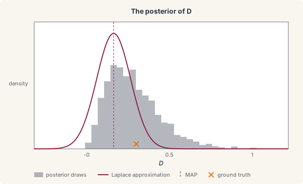
Instead, we can sample from the full posterior using Markov chain Monte Carlo methods provided by blackjax. We can draw samples from the full distribution in order to carry out a variety of uncertainty quantification tasks: assign credible intervals to each parameter, compute posterior means and correlations, propagate the parameter uncertainty to a band around the predicted solution, and carry it through the coefficients of a parameterized function (function approximation) to a band around the function itself. In this page we describe the process of posterior sampling in diff-soup and the typical workflows for PDE inference problems. The full sampling run:

spec = ds.problem("adsorption")
spec.domain("rod", cartesian_grid_1d(n, 0.0, 1.0, method="fvm"))
spec.field("u", mass="differential", scale=1.0, init=lambda x: x)
D = spec.param("D", value=0.1, learnable=True, bounds=(0.01, 2.0),
               prior=ds.inference.NormalPrior(mean=0.3, scale=0.3))        # the learnable diffusivity and its prior
a = spec.param("a", value=0.5, learnable=True, bounds=(0.0, 5.0),
               prior=ds.inference.NormalPrior(mean=1.0, scale=1.0))        # the learnable adsorption rate and its prior


@spec.equation(writes="u", reads=("u",))
def adsorption(q):
    return q.p.D * q.ops.laplacian(q.u) - q.p.a * q.u / (1.0 + q.u)


spec.bc.dirichlet("u", node_indices=np.array([0]), value=0.0)
spec.bc.dirichlet("u", node_indices=np.array([n - 1]), value=1.0)
problem = spec.build()
y0 = spec.assemble_state({})

measurement = ds.inference.Measurement("u", times=ts, values=data,
                                       likelihood=ds.inference.Gaussian(sigma=1e-1))
experiment = ds.inference.Experiment(model=problem, solver=solver, t_span=(0.0, 1.5),
                                     initial_state=y0, measurements=(measurement,))
est = ds.inference.InferenceProblem(experiment, parameters=(D, a), objective=ds.inference.MAP())   # the MAP problem
fit = ds.inference.optsolve(est, ds.inference.LevenbergMarquardt())                            # its mode

draws = ds.inference.sample(est, fit, key=jax.random.PRNGKey(0), chains=2, draws=1000, warmup=300)   # draw from the posterior
report = ds.inference.mcmc_report(draws)                                                 # check the draws
draws[D]                                                                                 # the draws of D

Sampling the posterior

To sample the posterior, we run a sampler on the MAP problem and its fit with ds.inference.sample, and check the draws with ds.inference.mcmc_report.

Run the sampler

ds.inference.sample(problem, fit, *, kernel="nuts", chains=4, draws=1000, warmup=200, adapt="pooled", mass="diag", step_size=None, max_tree_depth=10, key, preconditioner="laplace", curvature="observed", nuts_target_acceptance=0.8, chain_map=None) runs one chain per chains on the posterior of the MAP problem and returns the draws. An MLE problem is refused, since it has no prior.

draws = ds.inference.sample(est, fit, key=jax.random.PRNGKey(0), chains=2, draws=1000, warmup=300)

• fit is the MAP fit the chains start from.
• key is the random key. The same key reproduces the same draws.
• kernel="nuts" is the No-U-Turn sampler and the default. It follows the gradient of the posterior and adapts its step size and scale during the warmup. kernel="rmh" is the random-walk Metropolis kernel, which proposes Gaussian steps of a fixed size and needs no gradient. Any other name is refused.
• chains= is the number of chains. Each starts from the fit plus random noise of half a standard deviation of the Laplace approximation per coordinate (half a unit without the preconditioner below), so the starts lie inside the posterior.
• draws= is the number of draws kept per chain, and warmup= the number of steps before them. The random-walk chains discard their warmup steps. NUTS chains adapt during them and keep their last state, so the kept draws start adapted.
• adapt= is how NUTS adapts. "pooled" adapts one step size and one mass matrix from all chains at once, with the ChEES method of Hoffman et al. (2021) (references), so no single chain's noise sets them. "window" adapts each chain on its own with Stan's window schedule. "step_size" adapts only the step size and keeps the unit scale of the Laplace preconditioner, and None runs at step_size. One chain, or chains that do not run as one batched call, adapt as "window".
• mass="diag" adapts a diagonal mass matrix. "dense" adapts a full one, with adapt="window" and at most 50 parameters.
• step_size= is the step size adaptation starts from, 1.0 when None, and the fixed one with adapt=None. max_tree_depth=10 is the most times a NUTS trajectory doubles in one draw.
• preconditioner="laplace" scales the proposals of either kernel by the Laplace approximation of standard errors and covariance, so that the chains move at the width of the posterior from the first step. None runs the chains without it.
• curvature="observed" is the default curvature of that Laplace approximation. "expected" uses the expected curvature instead.
• nuts_target_acceptance=0.8 is the acceptance rate NUTS adapts its step size toward during the warmup.
• chain_map= places the chains. The default runs them as one batched call. "sequential" runs them one after another. "devices" places whole chains on the local devices, with chains a multiple of the device count. draws.chain_map records the placement that ran.
• A parameter with bounds is sampled in an unbounded coordinate, and every draw is returned in the parameter's own coordinate.

Analyze the draws

The draws are returned in the parameters' own coordinate, one array over the chains, the draws, and the parameters, and draws[D] returns the draws of one parameter.

draws.values.shape       # (2, 1000, 2), the chains, the draws, and the parameters
draws[D]                 # the draws of D, over the chains and the draws
draws.names              # the parameter labels
draws.info               # the acceptance rate and, for NUTS, the divergences per draw
predictive = ds.inference.predict(est, draws, kind="predictive")["u"]   # the solution over the draws, with noise

• draws.values holds the draws and draws.names labels them. draws[D] returns the draws of one parameter, and a dictionary by cluster for a parameter that varies by cluster (hierarchical fits).
• draws.info holds one value per draw of acceptance_rate, and for NUTS is_divergent and num_integration_steps. For NUTS, draws.info["adaptation"] records the method that ran, the adapted step_size of each chain, the mass, the max_tree_depth, the warmup and the mean acceptance_rate of the kept draws.
• ds.inference.predict(problem, draws, kind=) solves the model at every draw and summarizes the predicted values, the sampled counterpart of the prediction bands.

Whether the draws represent the posterior is the question of diagnostics, checked before any summary is taken.

Diagnostics

A chain represents the posterior only once it has forgotten its starting point and visited the posterior in proportion to its density, and a finite number of correlated draws carries less information than the same number of independent ones. ds.inference.mcmc_report(draws, *, rhat_max=1.01, ess_floor=400.0) checks both and flags the failures in words. Each chain needs at least eight draws.

report = ds.inference.mcmc_report(draws)
report.rhat              # near one when the chains agree
report.ess_bulk          # the number of independent draws the chains are worth
report.flags             # the failed checks in words, empty here
report.ok                # whether every check passed, True here
print(report.summary())  # the table of the above

• rhat compares the spread within each chain to the spread between them, per parameter, and is near one when the chains agree. It is flagged above rhat_max.
• ess_bulk and ess_tail are the effective sample sizes for the center and for the tails of the posterior, the number of independent draws the chains are worth. Each is flagged below ess_floor.
• mean, sd, and mcse_mean are the posterior mean, the posterior standard deviation, and the Monte Carlo error of the mean, per parameter.
• acceptance_rate and acceptance_rate_per_chain summarize the proposals, and for NUTS n_divergent, divergences_per_chain, tree_depth_max, and tree_depth_mean summarize the integration.
• flags lists the failed checks, ok is True when it is empty, and summary() renders a table of the above as text.

The diagnostics are the rank-normalized split \(\hat R\) and effective sample sizes of Vehtari et al. (2021) (references).

Preconditioning

The random-walk kernel steps with a fixed size, so it moves well only in a coordinate where the posterior has unit scale, and NUTS adapts faster from one. The default preconditioner="laplace" builds that coordinate from the Laplace approximation of standard errors and covariance, the affine map \(w \mapsto c + A w\) with \(c\) the mode and \(AA^\top\) the covariance, and runs the chains in \(w\). A Laplace approximation with an undetermined direction, from ds.inference.laplace(on_singular="subspace"), cannot precondition the chains (identifiability). For example, the random-walk kernel with and without it:

draws_rmh = ds.inference.sample(est, fit, key=jax.random.PRNGKey(0), kernel="rmh",
                                chains=2, draws=300, warmup=100)
draws_raw = ds.inference.sample(est, fit, key=jax.random.PRNGKey(0), kernel="rmh",
                                chains=2, draws=300, warmup=100, preconditioner=None)
ds.inference.mcmc_report(draws_rmh).acceptance_rate      # the fraction of proposals accepted
ds.inference.mcmc_report(draws_raw).acceptance_rate

Credible bands for fitted functions

A learnable function of function approximation is fitted through its coefficients, so its draws are coefficient vectors, and a credible band for the function follows by evaluating it at every draw. For example, with the diffusivity of the adsorption model allowed to vary along the rod as a Legendre expansion:

from diff_soup.inference.approx import Legendre

spec_f = ds.problem("adsorption_function")
spec_f.domain("rod", cartesian_grid_1d(n, 0.0, 1.0, method="fvm"))
spec_f.field("u", mass="differential", scale=1.0, init=lambda x: x)
D_of_x = spec_f.function("D_of_x", Legendre(jnp.array([np.log(0.3), 0.0, 0.0]), interval=(0.0, 1.0),
                                             transform=lambda x, p: jnp.exp(p)),
                         learnable=True, prior=ds.inference.GaussianCoefficientPrior(scale=1.0))   # a diffusivity along the rod and its prior
a_f = spec_f.param("a", value=0.5, learnable=True, bounds=(0.0, 5.0),
                   prior=ds.inference.NormalPrior(mean=1.0, scale=1.0))


@spec_f.equation(writes="u", reads=("u",))
def adsorption_f(q):
    return q.ops.div_flux(q.fn.D_of_x(q.x[:, 0]), q.u) - q.p.a * q.u / (1.0 + q.u)


spec_f.bc.dirichlet("u", node_indices=np.array([0]), value=0.0)
spec_f.bc.dirichlet("u", node_indices=np.array([n - 1]), value=1.0)
problem_f = spec_f.build()
est_f = ds.inference.InferenceProblem(
    ds.inference.Experiment(problem_f, solver, (0.0, 1.5), spec_f.assemble_state({}), (measurement,)),
    parameters=(D_of_x, a_f), objective=ds.inference.MAP())
fit_f = ds.inference.optsolve(est_f, ds.inference.LevenbergMarquardt())
draws_f = ds.inference.sample(est_f, fit_f, key=jax.random.PRNGKey(0), chains=2, draws=500, warmup=300)

coeffs = draws_f[D_of_x].reshape(-1, 3)                                              # one coefficient vector per draw
xs = jnp.linspace(0.0, 1.0, 101)
curves = jax.vmap(lambda c: Legendre(c, interval=(0.0, 1.0), transform=lambda x, p: jnp.exp(p))(xs))(coeffs)   # D(x) at every draw
lower, upper = jnp.percentile(curves, jnp.array([2.5, 97.5]), axis=0)                # the pointwise 95% credible band

• draws[handle] on a function handle returns the draws of its coefficients, one row per draw after the reshape, in the order of the expansion.
• The band is pointwise, one interval per position, and the same percentiles over curves give the band of any transform of the function.

References

• A. Vehtari, A. Gelman, D. Simpson, B. Carpenter, and P.-C. Bürkner. Rank-normalization, folding, and localization: an improved \(\hat R\) for assessing convergence of MCMC (with discussion). Bayesian Analysis, 16(2):667–718, 2021. doi:10.1214/20-BA1221.
• M. D. Hoffman, A. Radul, and P. Sountsov. An adaptive-MCMC scheme for setting trajectory lengths in Hamiltonian Monte Carlo. Proceedings of AISTATS, PMLR 130:3907–3915, 2021. proceedings.mlr.press/v130/hoffman21a.