Data assimilation

This page provides an overview of assimilating image data into a modeling and inference workflow. The running example is a set of image frames frames of a diffusing field on an oval, taken at the times ts, with square pixels of side pixel_size and the pixels outside the oval holding NaN.

Projecting image data onto a mesh

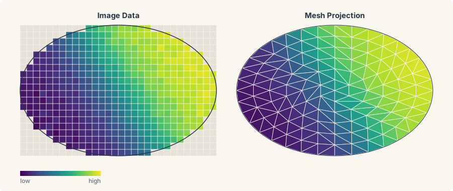
diff-soup provides operators for moving data between image space and a finite-element mesh. The binary mask of the domain, True on the oval and False elsewhere, is meshed with mask_to_mesh, a frame is projected onto the mesh nodes with interpolate_image_to_nodes, and PixelAveragingOperator maps a nodal field back to the pixels.

from diff_soup.domains.geometry import mask_to_mesh
from diff_soup.inference.data import PixelAveragingOperator, interpolate_image_to_nodes

mask = np.isfinite(frames[0])                                    # True on the oval
mesh = mask_to_mesh(mask, mesh_size=0.05, pixel_size=pixel_size)     # triangles inside the oval
pixel_origin = (pixel_size / 2, pixel_size / 2)                    # the center of pixel [0, 0]
u0 = interpolate_image_to_nodes(frames[0], mesh.points, pixel_origin=pixel_origin,
                                pixel_size=pixel_size, fill=0.0)   # the first frame at the nodes
op = PixelAveragingOperator.from_mesh_and_image(
    mesh.points, mesh.cells, image_shape=mask.shape, pixel_origin=pixel_origin,
    pixel_size=pixel_size, valid_mask=mask)
images = frames[:, mask]                                           # the observed pixels, one row per frame

• mask_to_mesh(mask, mesh_size=1.0, pixel_size=1.0, origin=(0.0, 0.0)) triangulates the region where the mask is True. mesh_size= is the triangle size in physical units, pixel_size= the side of one pixel, and origin= the physical position of the image corner. It needs the optional dependency gmsh.
• interpolate_image_to_nodes(image, points, pixel_origin=(0.0, 0.0), pixel_size=1.0, *, fill=None) gives one value per mesh node by interpolating between the pixels around it. pixel_origin= is the center of pixel [0, 0]. A node outside the image takes the nearest pixel. fill= replaces every non-finite pixel before interpolation, so the pixels outside the oval take fill=0.0 here; the default None propagates NaN.
• PixelAveragingOperator.from_mesh_and_image(points, cells, image_shape=, pixel_origin=, pixel_size=, valid_mask=None, ele_type="TRI3") builds the observation operator. op.predict(u) returns the pixels a nodal field predicts, in the order of images, and op.to_image(pixels) puts them back into an image.
• UpConvDownOperator.from_mesh_and_image(..., upscale=10) is the operator for a blurred image, with a one-pixel blur applied on a grid upscale times finer than the image. It needs matplotlib.

Estimating the initial condition

ds.inference.Experiment(..., initial_state=ds.inference.LearnedInitialState(guess), ...) fits the initial condition alongside the parameters, with guess the starting value of the state at the start of the experiment's span. A bare array stays a fixed state, and ds.inference.FixedInitialState(y0) is the explicit form. The fitted state reads back from result.window_states[0], or result.experiments[<id>].window_states[0], a (1, n_diff) block under single shooting and the first window block under a latent multishoot; both need optsolve(..., diagnostics=True), the default. Observed-state windows (Windows.from_data) refuse a learned state.

Interpolating boundary values

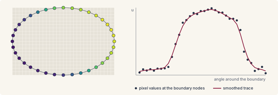
To directly impose Dirichlet boundary conditions from the image data, we provide extract_boundary_traces and smooth_boundary:

from diff_soup.inference.approx import PiecewiseLinear
from diff_soup.inference.data import extract_boundary_traces, smooth_boundary

boundary = mesh.boundary_nodes()
bc_raw = extract_boundary_traces(frames, mesh.points, boundary,
                                 pixel_origin=pixel_origin, pixel_size=pixel_size)
bc = smooth_boundary(bc_raw, mesh.points, boundary, c_lo=0.0, c_hi=1.0)
trace = PiecewiseLinear(ts, bc)                                    # one column per boundary node

• extract_boundary_traces(frames, points, boundary_indices, pixel_origin=, pixel_size=, fill_nan=None) returns one value per frame and boundary node. A NaN pixel takes fill_nan, or the frame's smallest finite value by default.
• smooth_boundary(bc_raw, points, boundary_indices, method="spline", c_lo=, c_hi=) smooths each frame around the contour and clips it to [c_lo, c_hi]. method="spline" fits a periodic smoothing spline with weights 1/sigma_eps (sigma_eps=0.01), method="savgol" applies a periodic Savitzky-Golay filter with window=7 and order=3, and method="raw" only clips.
• PiecewiseLinear(ts, values) turns the traces into a signal in time, passed as spec.bc.dirichlet(node_indices=boundary, value_fn=trace) (function approximation).

Fitting from the frames

The recipe takes the mesh as its domain and the trace as its boundary value. The operator's predict goes to ds.inference.Measurement(observe=), so the fit compares predicted pixels with the frames:

spec = ds.problem("heat_oval")
spec.domain("sheet", mesh)
spec.field("u", mass="differential", scale=1.0)
D = spec.param("D", value=0.1, learnable=True, bounds=(0.01, 2.0))


@spec.equation(writes="u", reads=("u",))
def heat(q):
    return q.p.D * q.ops.laplacian(q.u)


spec.bc.dirichlet("u", node_indices=boundary, value_fn=trace)
problem = spec.build()
y0 = spec.assemble_state({"u": u0})

measurement = ds.inference.Measurement("image", ts, images, observe=op.predict,
                                       weight=1e6)
experiment = ds.inference.Experiment(problem, ds.JIDA(), (float(ts[0]), float(ts[-1])), y0, (measurement,))
result = ds.inference.optsolve(ds.inference.InferenceProblem(experiment, parameters=D))
result[D]                                                          # the fitted diffusivity